i4Q Prescriptive Analysis Tools¶

General Description¶

i4QPA (Prescriptive Analysis Tools) is a micro-service consisting of simulation models as a service, taking as input the manufacturing resources, current production planning and process condition, and proposing process configuration parameters, ensuring that non-simulation experts may also exploit the prescriptive analyses.

i4QPA uses different data analytics platforms, thus allowing the evaluation and comparison of the results that come from the simulation of different industrial scenarios. i4QPA provides an extensive set of optimisation techniques that help in the development of the mathematical methods that will make the prescriptive analysis. These optimisation techniques have as objective the selection of the best of the digital twin instances that have been simulated, or even the selection of those simulation scenarios that need to be selected or avoided in order to reach faster the optimal solution, based on a scenarios map.

Features¶

This i4Q Prescriptive Analysis Tools offers following features:

Providing the capability of defining several scenarios to run simulations of the Digital Twin.
Providing the capability of defining custom optimization functions for evaluation and prescription of simulations’ results.
Providing the capability of defining the optimization functions and its inputs.
Providing tables and graph for an easy analysis of evaluation and prescription results.

Comercial information¶

Authors¶

Partner	Role	Website
IKERLAN	Leader	www.ikerlan.es/en/
EXOS	Vice-Leader	www.exos-solutions.com/
CERTH	Participant	https://www.certh.gr/root.en.aspx

Technical Specifications¶

i4QPA makes use of models (which can be generated by i4QDT) to test different possibilities and proposing process configuration parameters. First a set of possible scenarios needs to be defined. Then, they are simulated (with or without the support of the i4QDT). Finally, the results are evaluated and compared to provide a prescriptive analysis. The software solution can be containerized.

i4QPA allows to define different simulations to be performed (the scenarios) and its performance tested. For Digital Twins of the FMU type it uses the pyFMI package. In general, the communication with the Digital Twins can be managed through REST APIs provided by the i4QDT solution. This analysis can be visualized using a GUI generated using tools such as Shiny, Tkinter, Plotly.

i4QPA depends on i4QDT, as it supplies the simulation models. It may depend on some of the basic solutions (security, data traceability, …), it may also depend on the data integration and fusion micro-service, as well as the i4Q Data Repository. It may also give inputs to the i4Q Line Reconfiguration Toolkit.

Technical Development¶

This i4Q Solution has the following development requirements:

Development Language: Python and javascript.
Container and Orchestration: Docker
User Interface: React, PrimeReact, Redux.
Application Interfaces: RestAPI
Database engine: i4QDR
Python libraries: Numpy, Pandas, SciPy, Pywraplp, Pulp, Pickle.
Development Language: Python and javascript.
Libraries: Numpy, Pandas, PyYAML, FMPy, SciPy, XGBoost, Pickle.
Container and Orchestration: Docker.
User Interface: React, PrimeReact, Redux.
Application Interfaces: RestAPI.
Database engine: i4QDR.

License¶

Dual license AGPLv3 or PRIVATE.

Pricing¶

Subject	Value
Payment Model	Quotation under request
Price	Quotation under request

Associated i4Q Solutions¶

Required¶

The solution can operate without the need for another i4Q solution.

Optional¶

i4Q Digital Twin simulation services to carry out half of the simulations defined by i4Q Prescriptive Analysis Tools.
i4Q Data Repository and/or i4Q Data Integration and Transformation Services to get models’ inputs for simulation or evaluation.
i4Q Anaisis Dashboard for data and signal visulization.

System Requirements¶

The component may be run on any platform that support Docker images.

Installation Guidelines¶

The application can be found in the following link:

Resource	Location
Last release (v.1.0.0)	Gitlab Project

Being the repository files and folders structure as follows:

PA
    |-- orchestration
    |   |-- docker
    |       |-- docker-compose.yml
    |
    |-- subsystems
            |-- backend-python
            |   |-- Dockerfile
            |   |-- requirements.txt
            |   |-- src/public
            |       |-- config.yml
            |
            |-- frontend
            |    |-- Dockerfile
            |
            |-- PA_files
            |
            |-- docker-compose.yml

i4QPA docker installation¶

The Docker container of the application can be installed and launched following the next steps:

Install the Docker application.
Dowload the zip file from this link: Gitlab Project
Create a new folder in your local computer and extract the content of the zip file.
Configure the docker environment:

If the files availables for testing are to be used, move the folder “PA_files” to a working directory.
Open the “docker-compose.yml” file.
Indicate in “services/backend/volumes” in which folder the models, and custom evaluation functions, metrics and results are going to be stored (the “PA_files” folder’s working subdirectories or others).
Fmu files must either contain a valid linux binary dynamic library file or the source code so they can be automatically compiled by the library inside Docker.
Save and close the file.
Open the “config.yml” file.
Define the users custom predefined configuration (all users will start with the following configuration, but will be able to change it in the app): data_export, msg_broker, remote_storage and configuration.
Define simulations’ prefedined configuration.
Define the backend’s IP and port.
Save and close the file.
Open a new terminal in the folder where the “docker-compose.yml” file is located and run the following command:

docker-compose up --build

The application will be running as soon as the process finishes. The url where the user interface is running will be shown in the terminal, which by default is http://localhost:8082

User Manual¶

The use of the application’s user interface is optional, and so, the backend of the application can be accessed through API requests. In the following sub sections those API requests and the frontend are described.

API specification¶

The docker starts the backend server in the port 5000 and allows to use the following API methods. Those methods are accesible through the application frontend or sending the proper request using any other tool like Postman, or directly with Python code:

Resource	POST	GET
/models_information/names		Supported
/selected_model	Supported
/models_information/parameters		Supported
/submitted_parameters	Supported
/simulation_input	Supported
/simulation_information/model_configuration		Supported
/simulation_configuration	Supported
/simulation/start	Supported
/simulation/state		Supported
/simulation_results		Supported
/evaluation/information	Supported
/simulation/filter1/post		Supported
/evaluation/configuration	Supported
/evaluation/results		Supported

/models_information/names → Get a 3 level data-tree with the available models.
- The first level indicates the folder in which the models are saved whitin the folder indicated in the configuration. If the models are not saved in an specific folder, the models are grouped with the label “misc”.
- TThe second level indicates which type of model is: physics-based or data-driven (“data_driven”). Physics-based models can be single (“single”) or composed of 1 or more single models (“compound”).
- The third level indicates the models’ name and key. The key is used in the /selected_model POST request to select a model to work with.
/selected_model → Select the model to prescribe by means of the key.
- Request type:

{"selected_model": "2-0-1"}.

/models_information/parameters → Get the model’s internal parameters information.
/submitted_parameters → Set the range of the model’s internal parameters. The range can be indicated as a range or a couple of limits. The range will be added and substracted to the original value to calculate the limits.
- Request type:

{"0": {"name": "mass1.m", "valueReference": 25, "startValue": 50, "rangeValue": 2, "stepValue": 1},
"1": {"name": "mass2.m", "valueReference": 27, "startValue": 100, "downValue": 10, "upValue": 150, "stepValue": 1}}

/simulation_input → Send the files that contain the model’s input signals. If a new request is sent, all the previous files are deleted.
- Request type: “form-data”
- Key: “inputSignal[]”
- Value: “file”
/simulation_information/model_configuration → et the model’s map of scenarios created with the /submitted_parameters POST request’s data.
/simulation_configuration → end the simulations’ configuration. For serial simulations the “simulation_type” variable must be set as “0”, for parallel simulations to “1”.
- Request type:

{"simulation_type": 0, "simulation_cores": 2, "start_time": 0, "stop_time": 5, "step_size": 0.01}

/simulation/start → Start the simulations.
- Request type:

{"start_simulation": 1}

/simulation/state → Get the state of the simulations: the amount of simulations to be carried out, the current simulation time, … Only to be used with parallel simulations.
/simulation_results → Get the results of the simulations. f the message size is too big to be sent through GET request, data can be stored as an Excel in the defined path with the following request.
/simulation/filter1/post → Select which simulations and signals are wanted to be saved in an Excel.
- Request type:

{"simulationSelectedModelOutputs": ["x1", "x2"], "simulationSelectedSimulationsOutputs": ["0-20"], "simulationSelectedModelInputs": ["inputF"], "simulationSelectedSimulationsInputs": ["0"]}

/evaluation/information → Get a dictionary with all the predefined and custom evaluation functions.
/evaluation_input → Send signals files to be used with evaluations.
- Request type: “form-data”
- Key: “inputSignal[]”
- Value: “file”
/evaluation/configuration → Submit the configuration of the evaluation. The structure of this request is dependant of the evaluation functions saved in the folder indicated in the configuration of the solution. In the following line there is an example of a configuration, apart from the variables type of the example, the evaluation functions’ parameters can also be integers (“int”), floats (“float”) or boolean (“bool”):
- Request type :

{"functions": ["fcn_name1", "fcn_name2"],
"params": [["T1", 0, "1"], ["T2", 1]],
"name": [["signal", "objetive", "bigger_than"], ["signal", "objective"]],
"type": [["signal", "float", "bool"], ["signal", "float"]]}

/evaluation/results → Get the evaluation results. Each result dictionary relates to one specific simulation, and so, to one specific model scenario. Therefore, to prescribe the optimum model scenario, the results have to be sorted. If the evaluation results table is too big to be sent, the results can be obtained from the Excel that is created everytime the previous request is send.

Front-end User Manual¶

The application will open in one of its 4 tabs, the home tab precisely. The tabs navigation widget is placed in the left, and the available tabs are:

Home → Tab in which an introduction of i4QPA is displayed.
Configuration → Tab in which the aplication configuration can be changed.
Simulation → Simulations’ configuration and results visualization. This main tab contains three sub-tabs:
- The configuration sub-tab, where the simulations are configured, from the model selection, to the model scenarios.
- The filtering sub-tab, where the model scenarios table is displayed and the simulations’ results’ signals to be plotted can be selected.
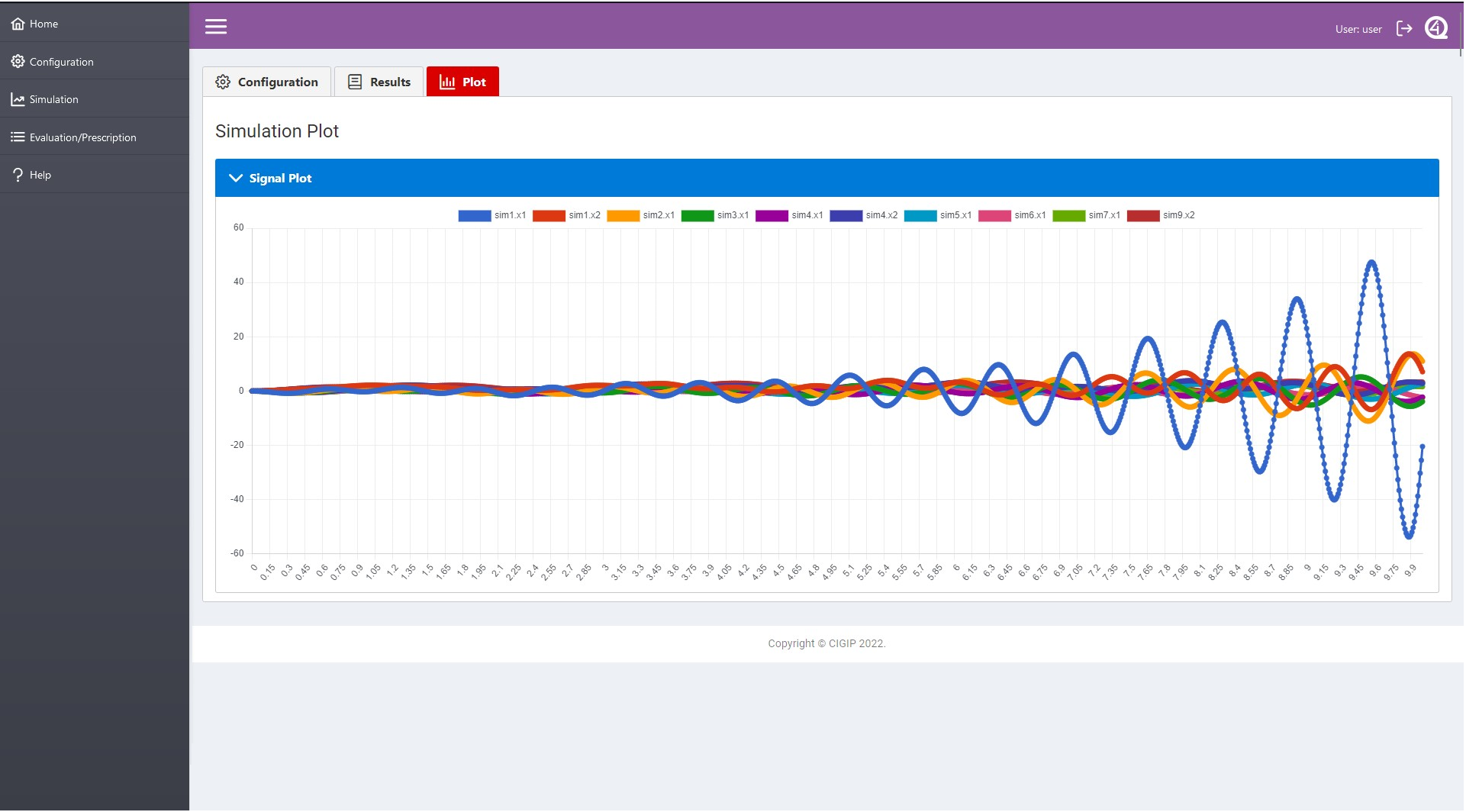
- The simulations’ results visualization tab, where the selected signals are displayed in a graph.
Evaluation/Prescription → Tab where the evaluation and prescription is configured and visualized. This main tab contains three sub-tabs:
- The configuration sub-tab, where the evaluations are configured, from the selection of evaluation functions, to the definition of the functions inputs.
- The results visualization sub-tab, where the evaluations results table is displayed and the prescription of the selected simulations/evaluation function can be visualized.
- The evaluations results plot, where the evaluation results are plotted as a bar graph.
Help → Tab with the guidelines to create custom metrics and evaluation functions.

The tabs “Configuration”, “Simulation” and “Evaluation/Prescription” cannot be accessed if not logged in. The login can be done by clicking in the top-right user button.

Resource	POST	GET
/models_information/names		Supported
/selected_model	Supported

Home	Configuration
Home	configuration
Simulation	Evaluation
SIM_CONF	evaluation
Help
help

Three type of models can be analized: single and compound physic-based models, and data-driven models. All three are analized similarly. The prescription process goes as follows:

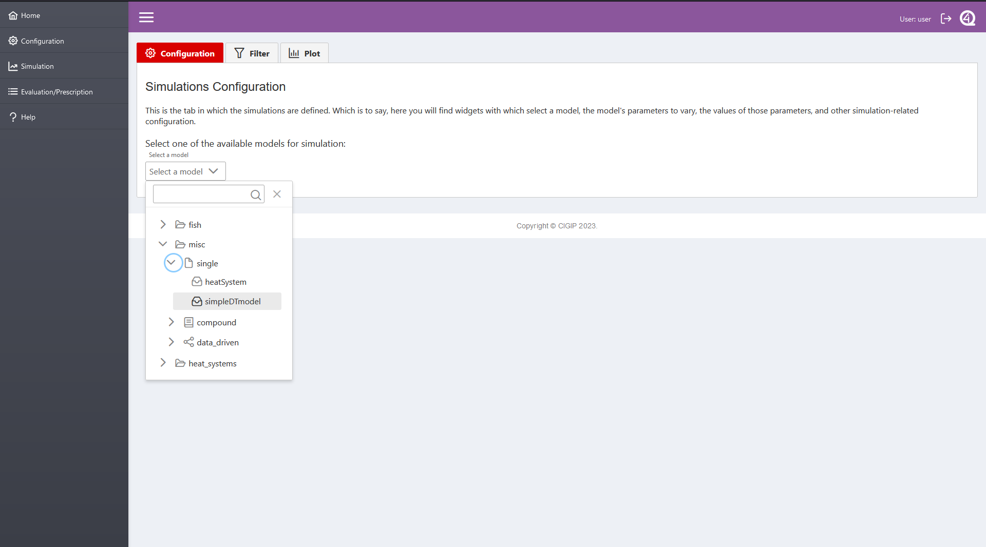
Open the simulation main tab
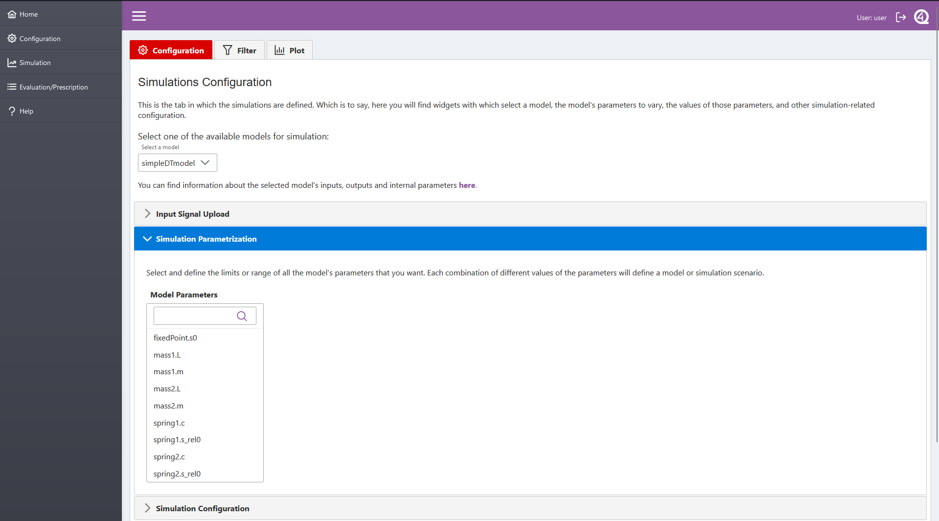
- Select a model in the 3 level data-tree widget (left image). When a model is selected, the internal parameters of the model are made available in the “Simulation Parametrization” drop-down widget (right image), if applicable.

Model Select¶

Model_Select Param configuration ———— Param

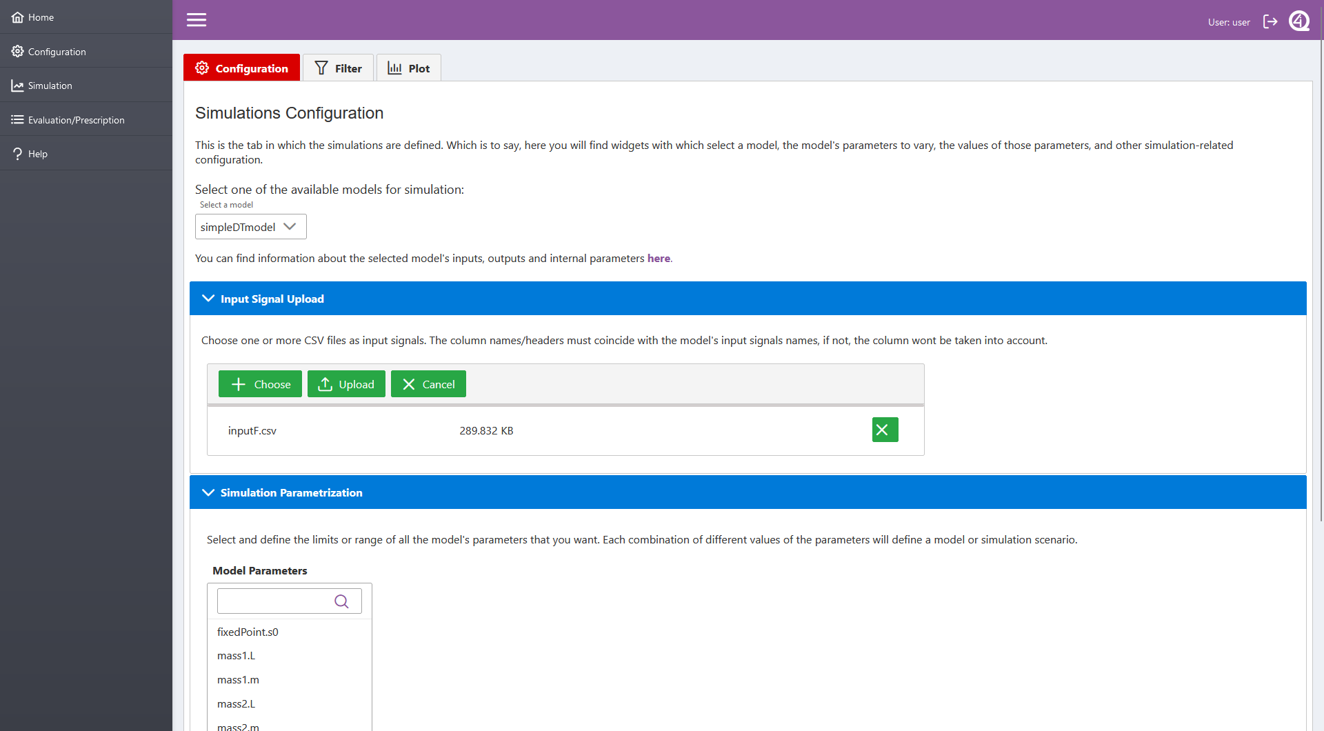
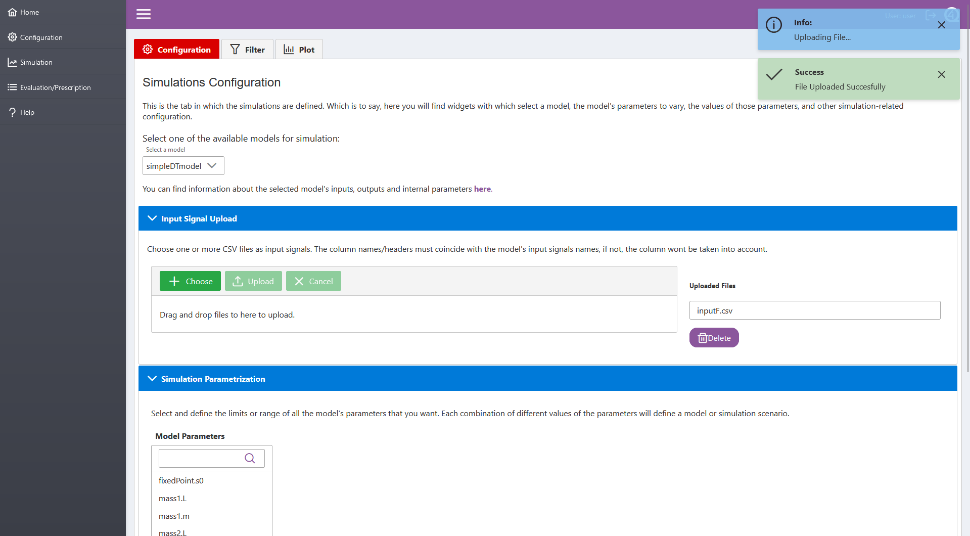
Define the simulations’ model scenarios with variations of the model’s input signals (“Input Signal Upload” drow-down widget) and/or internal parameters (“Simulation Parametrization” drop-down widget).

Input Signal Upload:

The “Choose” button opens a file browser in which the user can select csv files containing input signals (left image). More than one csv can be selected, but they have to be added/selected one by one.

The “Upload” button uploads the selected csv files’ signals (right image). The files must contain a header with the name of the signals, and those names must coincide with the model’s inputs names. If not, the signals are not uploaded.

Uploaded files can be deleted with the “Delete” button.

Choose Input¶

Choose_Input Upload Input ———— Upload_Input

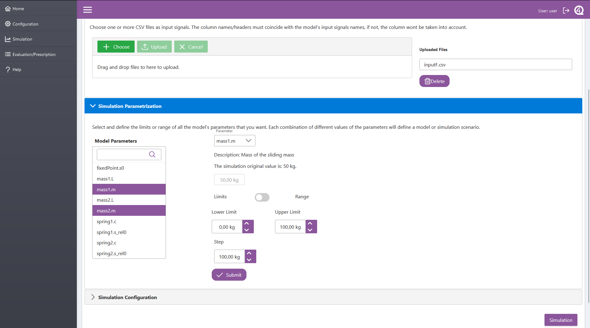
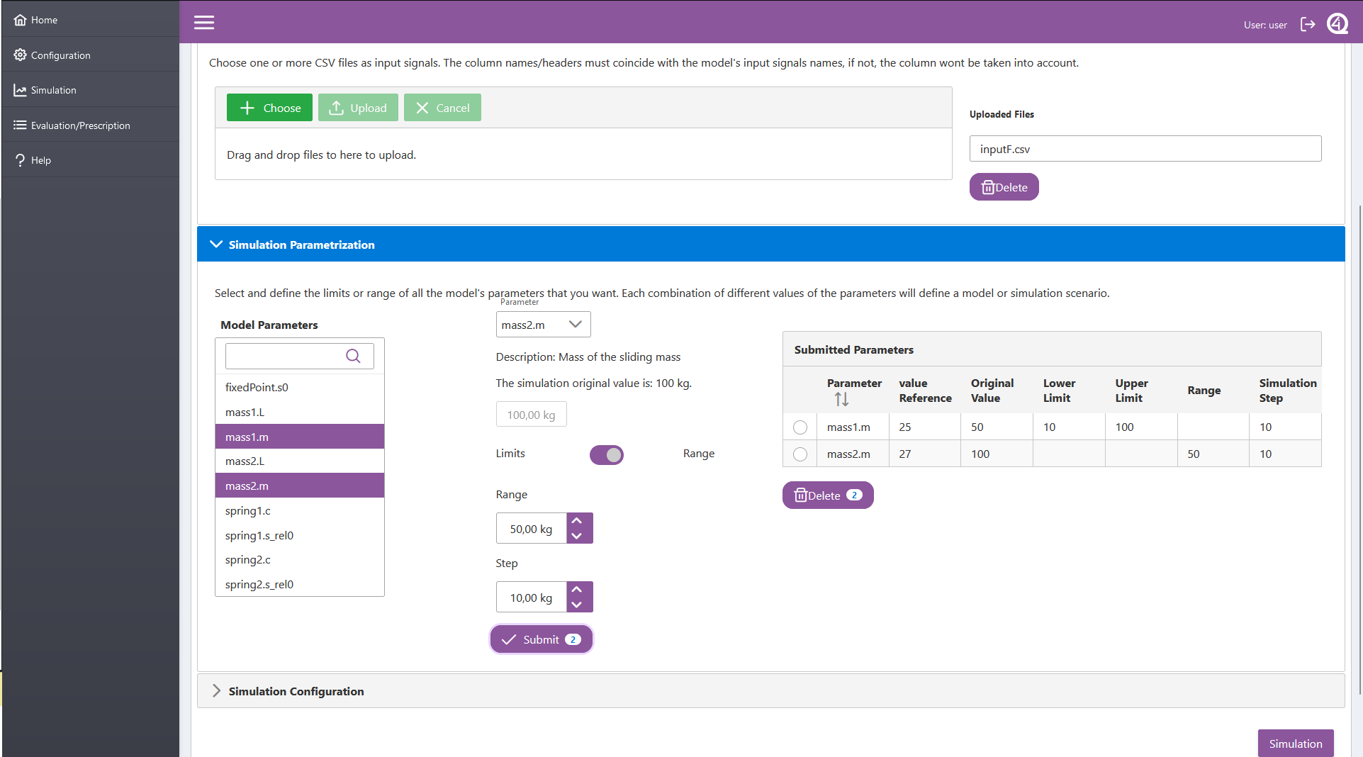
Simulation Parametrization:

Select all the parameters that are wanted to vary.

In the “Parameter” selector, select one of the parameters.

Define the parameter’s values by limits or range.

Limits: the user has to define the upper, lower and step value of the parameter (left image).

Range: the user has to define the range and step value of the parameter (right image). Which is to say, the lower limit is going to be the orignal value of the parameter minus the defined range, and so, the upper limit, the original value plus the range.

Press “Submit”.

Repeat the process with the other selected parameters.

Param Select¶

param_select Param Range Defined ——————– param_range_defined

Define the rest of simulation configurations in the “Simulation Configuration” drop-down widget.:

Start, stop and step time of the simulations.

Serial/parallel simulations state selector. If parallel is chosen, the number of cores have to be defined.

i4QDT simulations request state selector.

sim_config

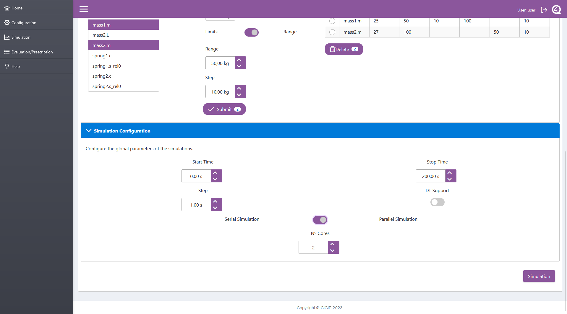
Press “Simulation” button. The frontend will move the user from the “Simulation/Configuration” tab to the “Simulation/Results” tab while the simulations are carried out. In the results tab the defined model scenarios are displayed in a table.

Simulations’ results can be plotted even if it is not required for the prescription proccess.

In the first filter (left image), select the inputs, outputs and simulations that are wanted to be plotted.

In the second filter (right image), select individual signals.

1st filter¶

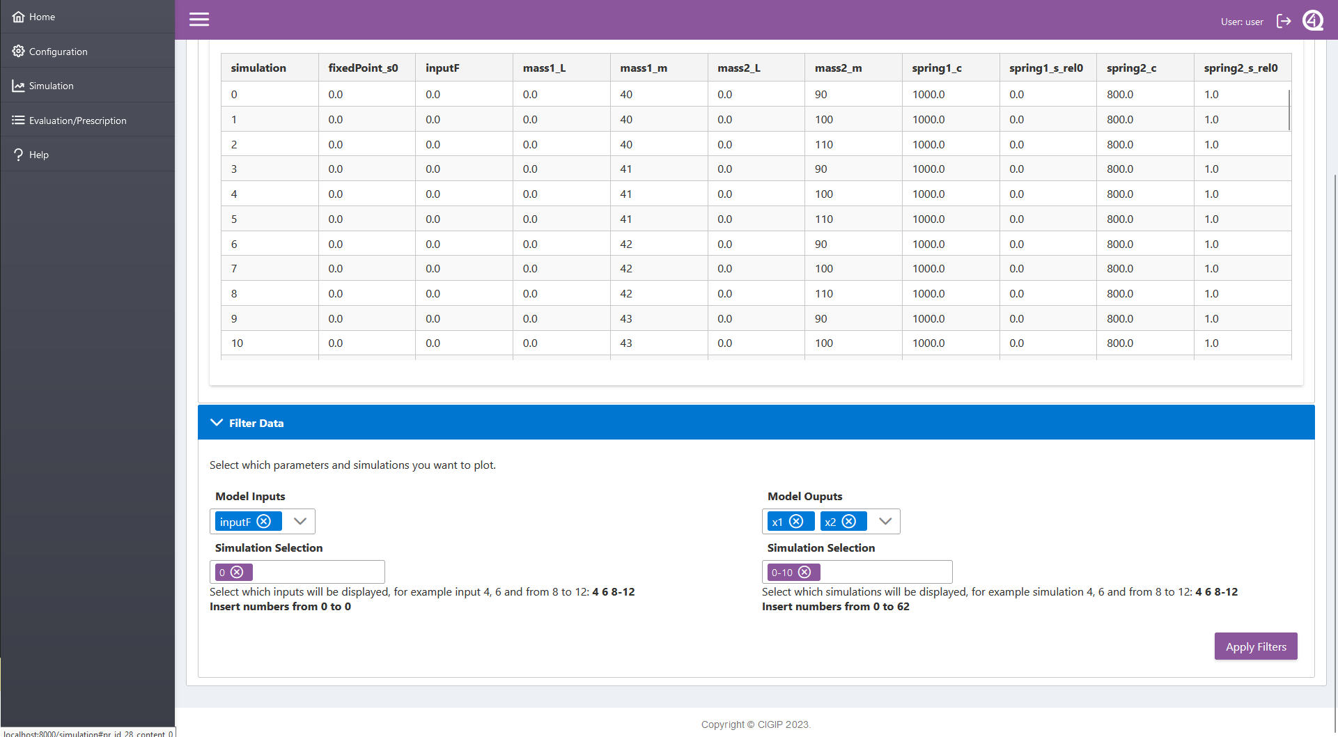1st_filter 2nd filter ———- 2nd_filter

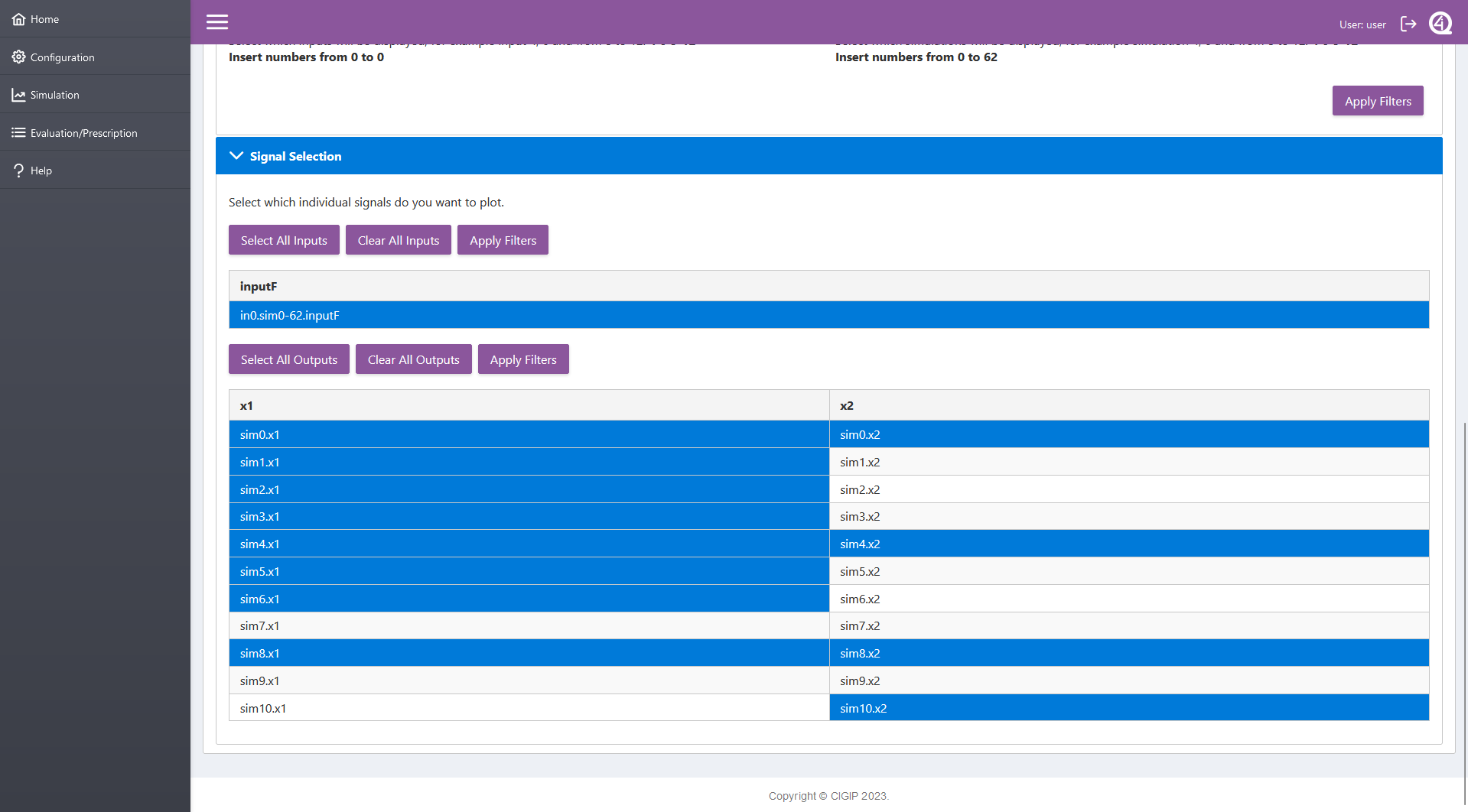
Press “Apply Filters”.

sim_results_plot

Move to the “Evaluation/Prescription” main tab.

Chose and add one or more evalution functions in the “Select an evaluation function” selector.

eval_fcn_select

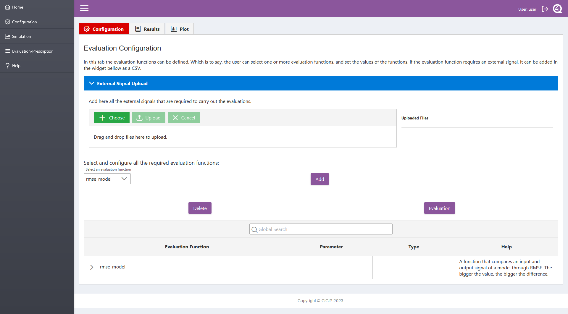
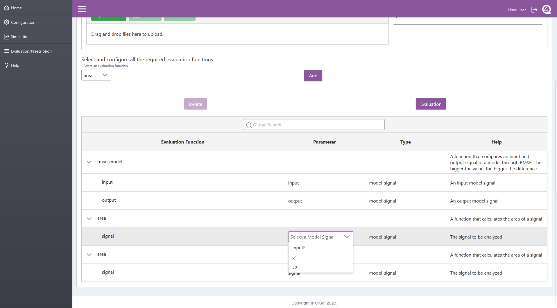
Define the evaluation functions parameters in the “Parameter” column of the table (left image). A help and type column has been added to help the user define the parameters. Depending on the type, a selector or a number input is going to be made available for the user.

“model_signal”: a model’s input or ouput signal. The options are limited through a selector.

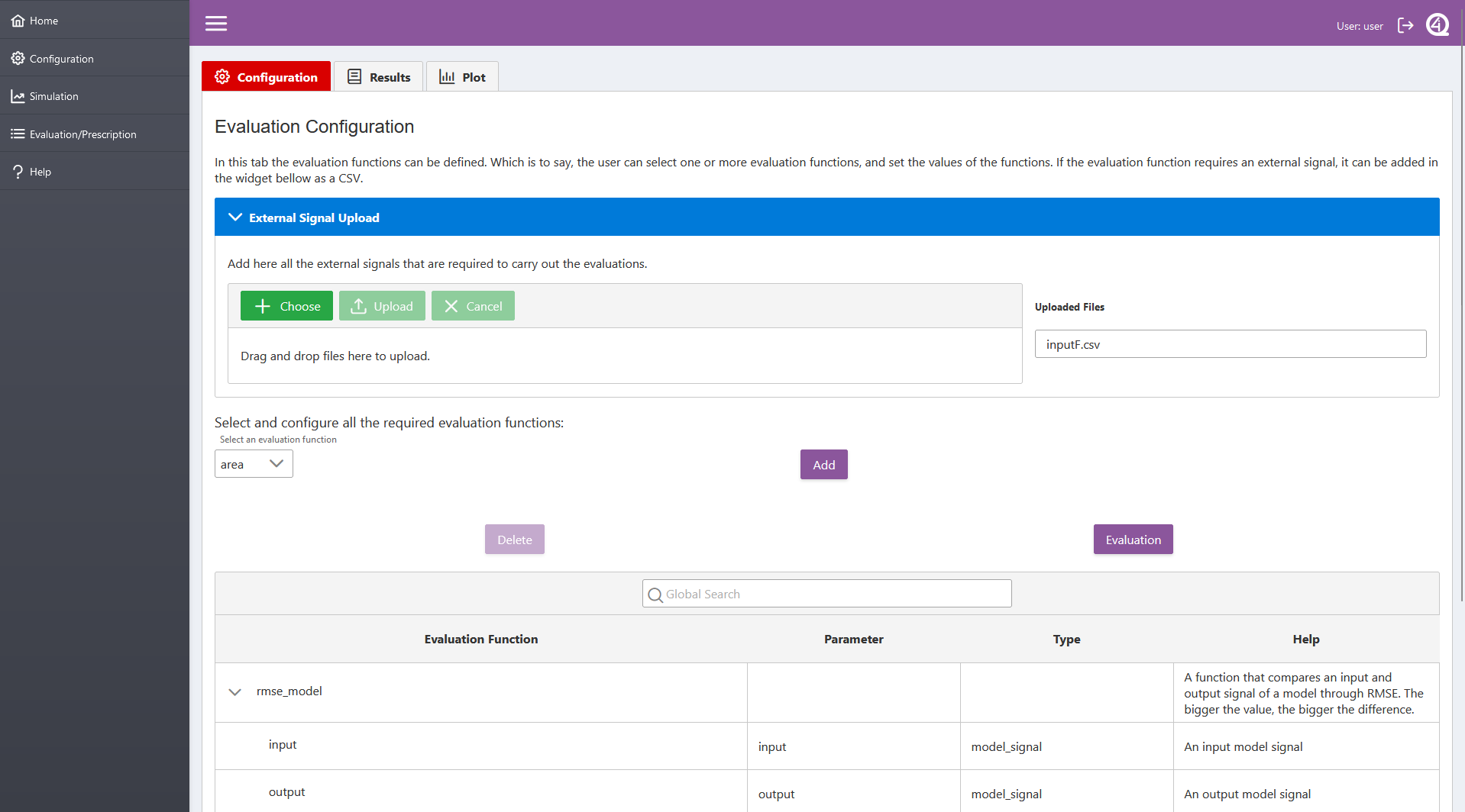
“ext_signal”: an external signal introduced in the “External Signal Upload” widget (right image). The options are limited through a selector.

“bool”, “int” and “float”.

Eval Fcn Params¶

eval_fcn_params Eval Fcn Ext Signal ——————- eval_fcn_ext_signal

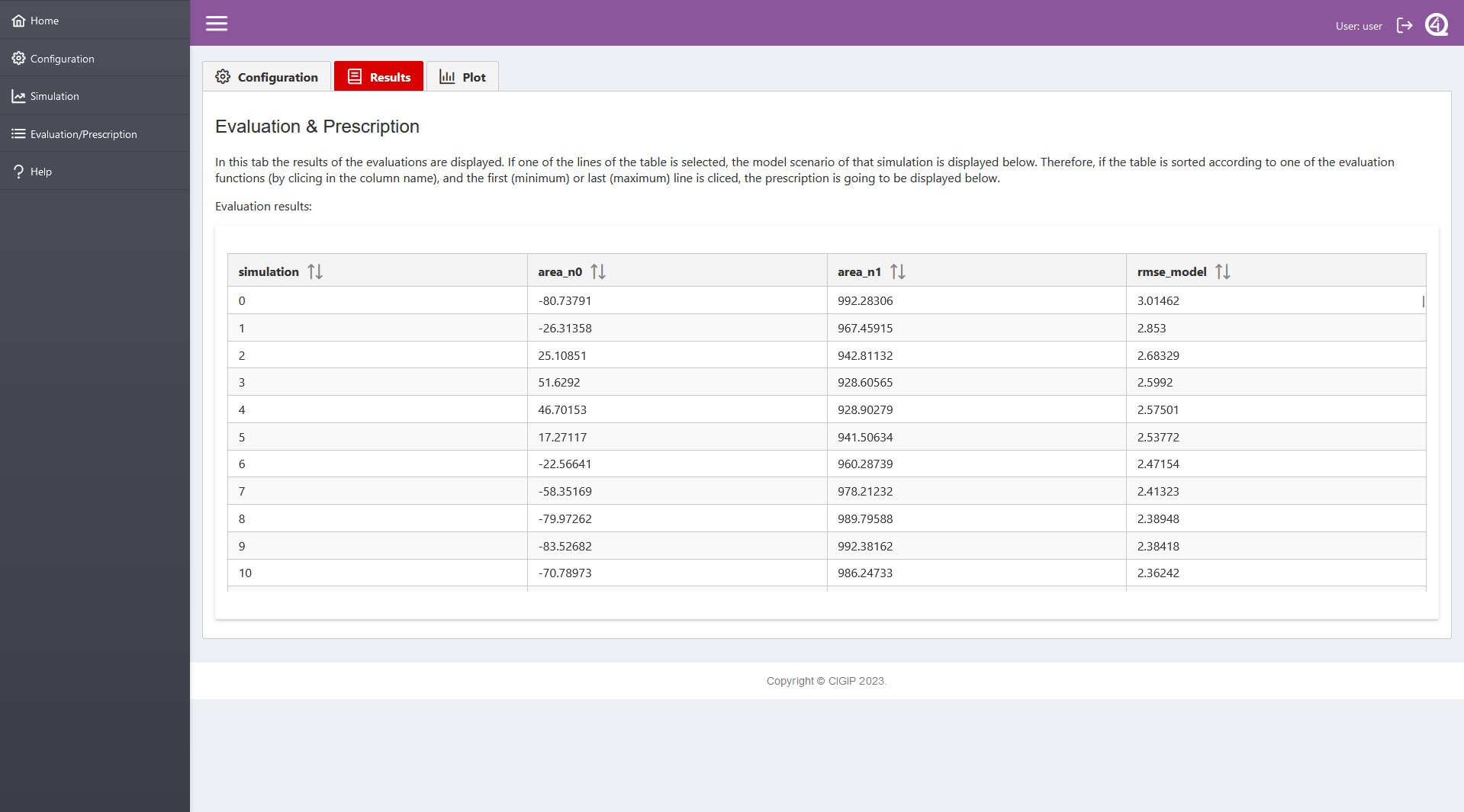
Press “Evaluation”. The user is moved to the “Results” sub-tab, where the evaluation results are displayed in a table.

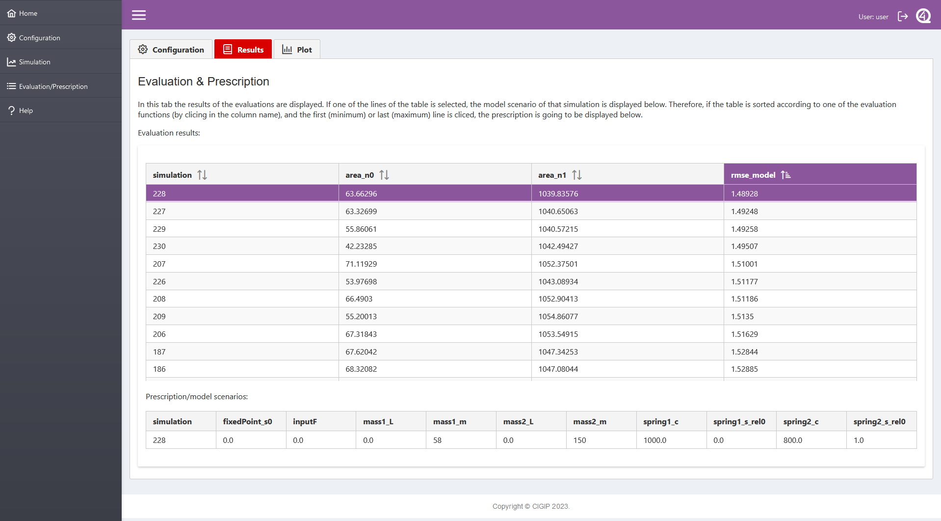
To prescribe the optimum system according to an specific evaluation function, the user has to:

Sort the table by clicking on the required evaluation function name.

Click on the first or last simulation of the sorted table, depending on if the user wants to minimize or maximize that specific evaluation result.

Check the model parameters of the prescription table below.

Eval Results¶

eval_results Prescription ————

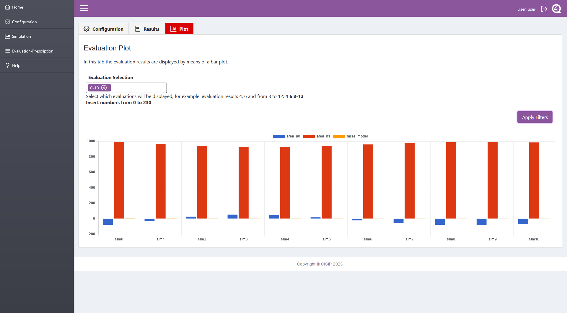
Evaluation results can be plotted in the “Evaluation/Prescription/Plot” tab.

Define the simulations whose evaluations results are wanted to be displayed.

Press “Apply Filters”.

eval_result_bar_plot